Design Of Experiment

 Design Of Experiment (DOE)

For this experiment we were tasked with applying what we learnt in class about full factorial and fractional factorial data and how to gather the data we need during the practical. For full factorial, 64 sets of data had be collected while for fractional factorial, only half were collected so, 32 sets. The experiment had involved launching a ball using a catapult and seeing how changing some factors would affect the projectile distance.

During the practical we were split into groups that were randomly generated. The groups were then split into two smaller groups which one group does data collection for full factorial design and the other does data collection for fractional factorial. I was in the group that was doing data collection for full factorial

Before beginning the data collection, we measured out all the factors that were being changed during the experiment.

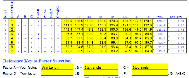
The factors being changed for each run were arm length, start angle, stop angle. The plus and minus represents the high level and low level of each factor respectively.

Full Factorial Design

For full factorial data, before we collected the data, we made a few precautions to ensure results were as accurate as possible. First, we did the testing on the floor as there would be more space and the ball used would not fall from a great height reducing the chance of the ball being damaged. Secondly, we tape the catapult to the ground to ensure that after each launch, the catapult would not move out of position. Lastly we had taped the measuring tape to the ground so that we can have accurate measurements of the projectile distance.

We then started the experiment, since both the full factorial and fractional factorial data collection were both done at the same time we had given roles to each member. The roles were one person launching both catapults ensuring the balls used for each catapult were the same each run, two recorders, records the projectile distance in the excel template, two people who measured the distance travelled in the sand patch by the ball. 

We did runs 2,3,5,8 first to match up with the fractional factorial group. The factors were changed according the excel template given. After finishing runs 2,3,5,8, we did runs 1.4.6.7 changing the factors for different runs and ensuring the ball used was not changed. All the runs had been repeated eight times. After collecting the data, the table would look something like this.

Then, we compared the averages of each factor when they are at high or low level and find the differences of the average to see the significance of each factor.

A graph is then plotted to see the difference in gradients and find out the significance of each factor.

The order of significance is as follows, stop angle (most significant), arm length, start angle (least significant)

From here we can start determining the interaction effects between each factor. To determine the interaction effect of each factor, we first pick out two factors. For this example we will pick factor A (arm length) and B (start angle) 

We need to compare the average values of A when factor B and A is both low and low level, low and high level respectively, high and low level respectively, high and high level. Using the table to get the average values for each run, the calculations looks like this,

Interaction between A and B:
Runs for low A and low B, run 1,5
Runs for high A and low B, run 2,6
Runs for low A and high B, run 3,7
Runs for high A and high B, run 4,8
At LOW B, Average of low A= (180.3+90.5)/2=135.4
At LOW B, Average of high A= (116.5+93.7)/2=105.1
At LOW B, total effect of A= (105.1-135.4) =-30.3 (decrease)
At HIGH B, Average of low A= (145.5+91.6)/2=118.55
At HIGH B, Average of high A= (88.5+83.5)/2=86

At HIGH B, total effect of A = (86-118.55)=-32.55

Using the values from the "total effect of A", a graph is plotted to find out the interaction,

The gradient of both lines represents the interaction and since the gradient of both lines have very little difference, the interaction between A and B is small.

Repeat these steps for A and C , and B and C

Interaction between A and C:

Runs for low A and low C, run 1,3

Runs for high A and low C, run 2,4

Runs for low A and high C, run 5,7

Runs for high A and high C, run 6,8

At LOW C, Average of low A= (180.3+145.5)/2= 162.9

At LOW C, Average of high A= (116.5+88.5)/2= 102.5

At LOW C, total effect of A= (102.5-162.9) = -60.4 (decrease)

At HIGH C, Average of low A= (90.5+91.6)/2= 91.05

At HIGH C, Average of high A= (93.7+83.5)/2= 88.6

At HIGH C, total effect of A= (88.6-91.05) =-2.45 (decrease)

The gradient of both lines are negative and are different. Therefore, there is a significant interaction between A and C

Interaction between B and C:

Runs for low B and low C, run 1,2

Runs for high B and low C, run 3,4

Runs for low B and high C, run 5,6

Runs for high B and high C, run 7,8

At LOW C, Average of low B= (180.3+116.5)/2= 148.4

At LOW C, Average of high B= (145.5+88.5)/2= 117

At LOW C, total effect of B= (117-148.4) = -31.4 (decrease)

At HIGH C, Average of low B= (90.5+93.7)/2= 92.1
At HIGH C, Average of high B= (91.6+83.5)/2= 87.55

At HIGH C, total effect of B= (87.55-92.1) =-4.55 (decrease)

The gradient of both lines are negative and different. Therefore, there is a significant interaction between B and C.

Link to excel file

https://docs.google.com/spreadsheets/d/1HrrfXxuk22XEuaqpBuwFaM9Q9iyaqjyw/edit?usp=sharing&ouid=110392842681122761336&rtpof=true&sd=true

Conclusion

Using full factorial would provide more data and lead to more accurate results but it is definitely slower and more tedious to obtain all the results compared to fractional factorial design. The calculations for the interaction effects is also more complicated as there is more steps but, nevertheless, calculations would be more accurate. To have the highest projectile distance, set all factors to low level.

Fractional Factorial Design

The testing was done concurrently with the full factorial design hence the precaution taken was the same. Only runs 2,3,5,8 were done and the data was recorded hence the table would look like this, The factors that were being monitored were also the same.

Just like the full factorial design, the data is calculated to find the significance of each factor

The graph is then plotted 

The order of significance is as follows, stop angle (most significant), arm length, start angle (least significant)

The result is the same as the data in full factorial design data.

The interaction effect can now be compared, since there is only half the runs the calculations are shorter and less complicated. Comparing factor A and B as the first example.

Interaction between A and B

At LOW B, Average of low A= 101.5 (run 5)
At LOW B, Average of high A = 134.0 (run 2)

At LOW B, total effect of A= (134-101.5) =32.5 (increase)
At HIGH B, Average of low A = 154.7 (run 3)

At HIGH B, Average of high A = 81.0 (run 8)

At HIGH B, total effect of A= (81-154.7) =-73.7 (decrease)

The gradient of both lines is different (one is + and the other is -). Therefore, there is a significant interaction between A and B.

Repeat these steps for A and C , and B and C

Interaction between A and C:

At LOW C, Average of low A= 154.7 (run 3)
At LOW C, Average of high A= 134 (run 2)

At LOW C, total effect of A= (134-154.7) = -20.7 (decrease)
At HIGH C, Average of low A= 101.5 (run 5)

At HIGH C, Average of high A= 81 (run 8)

At HIGH C, total effect of A= (81-101.5) =-20.5 (decrease)

The gradient of both lines is different by a little margin. Therefore, there is an interaction between A and C, but the interaction is small.

Interaction between B and C:

At LOW C, Average of low B= 134 (run 2)
At LOW C, Average of high B= 154.7 (run 3)
At LOW C, total effect of B= (154.7-134) = 20 (increase)
At HIGH C, Average of low B= 101.5 (run 5)
At HIGH C, Average of high B= 81 (run 8)

At HIGH C, total effect of B= (81-101.5) =-20 (decrease)

The gradient of both lines is different (one is + and the other is -). Therefore, there is a significant interaction between B and C.

Link to excel file: ``

https://docs.google.com/spreadsheets/d/1VvAy8AgRvU1jKBFngVpS2uhkL5xaqqP8/edit?usp=sharing&ouid=110392842681122761336&rtpof=true&sd=true 

Conclusion

Fractional factorial is much faster to carry out and less complicated when it comes to calculation for the interaction effect between factors as compared to the full factorial. However it would be less accurate as compared to full factorial. But, it would be more useful more situations where given resources can only collect 16 data points for example. Using fractional factorial would allow us to collect four data points while full factorial would only allow us to collect two data points. To have the highest projectile distance, set arm length to low level, start angle to high level and, stop angle to low level.

Case Study:

After having the practical, a task is given to the group and different case studies are done by different members of the group depending on their roles. Since I am the chief safety officer, case study 2 is assigned to me and is solved by using the fractional factorial method. 

The context of the case study is,

In a waste water treatment facility, a combination of coagulant chemicals, treatment temperature and stirring speed were identified as a critical factor to treat the waste-water to produce clean water. The clean water produced is recycled back into the main proses and at the same time reduce the amount of pollutant discharged by the plant. 

8 runs were performed and the data are shown below. 

The response variable (y) is the amount of pollutant discharged (lb/day) 

A = concentration of coagulant added, 1% and 2% by weight 

B = treatment temperature, 72o F and 100o F 

C = Stirring speed, 200 rpm and 400 rpm

Using the excel template, the average value, y (lb/day) is filled in the table and the average is calculated. Since fractional factorial design is used, runs 2,3,5,8 is used.

The average is then calculated so that we can find the significance of each factor.

Then, the graph is plotted,

The order of significance is as follows, stirring speed (most significant), coagulant concentration being equally significant as treatment temperature.

The interaction can now be calculated to find about the interaction effect of each factor. Comparing factor A and B for the first example.

Interaction between A and B

At LOW B, Average of low A= 4 (run 5)
At LOW B, Average of high A = 30 (run 2)

At LOW B, total effect of A= (30-4) =26 (increase)
At HIGH B, Average of low A = 6 (run 3)

At HIGH B, Average of high A = 4 (run 8)

At HIGH B, total effect of A= (4-6) =-2 (decrease)

The gradient of both lines is different (one is + and the other is -). Therefore, there is a significant interaction between A and B.

Repeat these steps for A and C , and B and C

Interaction between A and C:

At LOW C, Average of low A= 6 (run 3)
At LOW C, Average of high A= 30 (run 2)

At LOW C, total effect of A= (30-6) = 24 (increase)
At HIGH C, Average of low A= 4 (run 5)

At HIGH C, Average of high A= 4 (run 8)

At HIGH C, total effect of A= (4-4) =0 (no change)

The gradient of both lines is different (one is + and the other is a horizontal line). Therefore, there is a significant interaction between A and C.

Interaction between B and C:

At LOW C, Average of low B= 30 (run 2)
At LOW C, Average of high B= 6 (run 3)
At LOW C, total effect of B= (6-30) = -24 (increase)
At HIGH C, Average of low B= 4 (run 5)
At HIGH C, Average of high B= 4 (run 8)

At HIGH C, total effect of B= (81-101.5) =-20 (decrease)

The gradient of both lines is different (one is - and the other is a horizontal line). Therefore, there is a significant interaction between A and C.

Link to excel file: ``

https://docs.google.com/spreadsheets/d/1jZxrhcY61YUCbLi0KZA60v4RA8hZzYqa/edit?usp=sharing&ouid=110392842681122761336&rtpof=true&sd=true

Conclusion

To get the highest pollutant discharged, set the coagulant concentration to high level, treatment temperature to low level, and stirrer speed to low level.